What Is KV Cache? A Plain-English Guide for LLM Inference

A KV cache stores the key and value vectors an LLM already computed for the tokens in a sequence, so the model reuses them instead of recomputing them on every step. It is one of the biggest reasons self-hosted LLM inference is fast enough to ship.

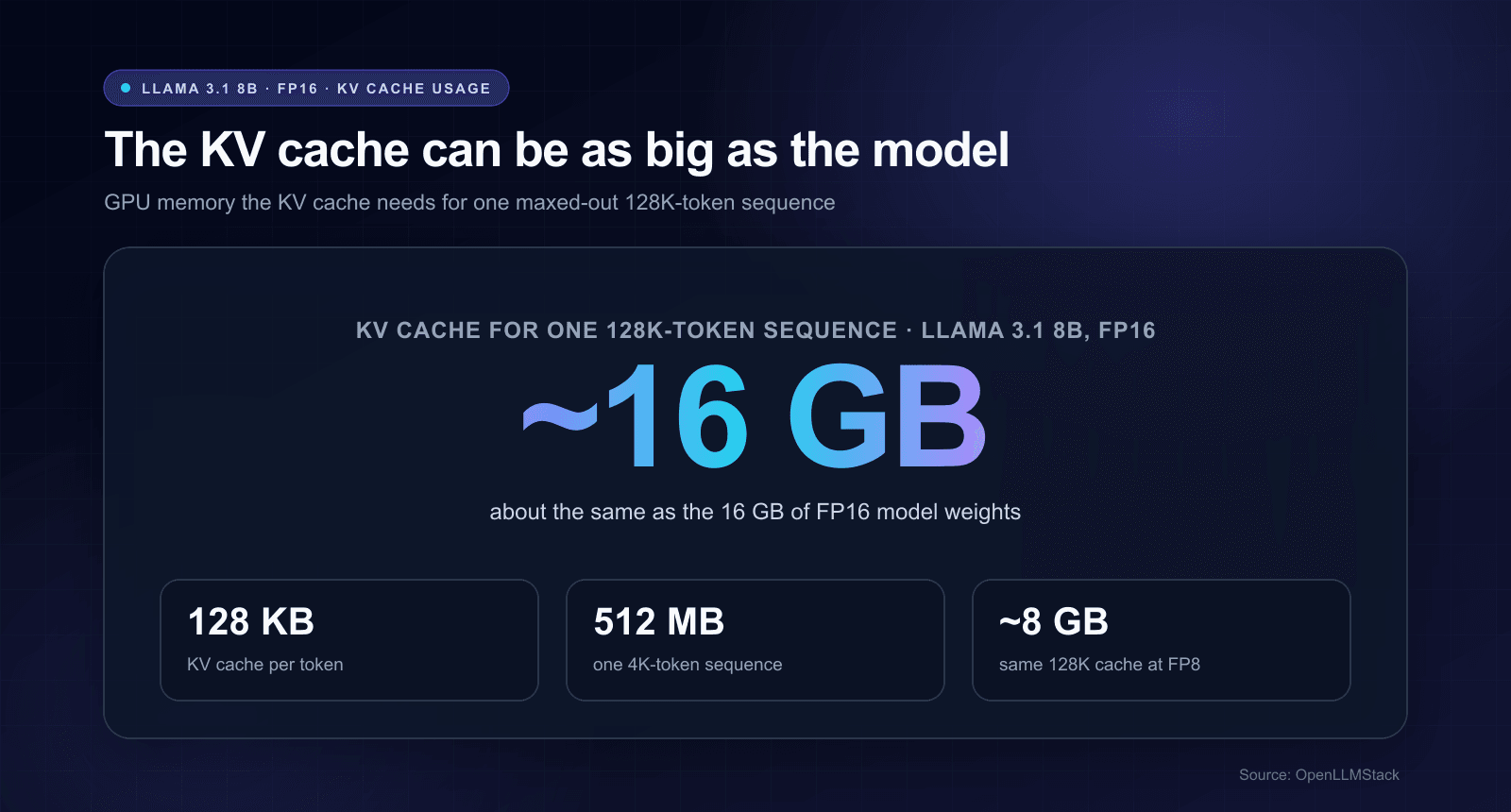
However, that speed is not free. The KV cache can eat more GPU memory than the model weights themselves, especially with long contexts or many concurrent requests.

This guide explains what a KV cache is, how it works, how to calculate the memory it needs, and how to shrink it. In plain English, with the math worked out.

The problem: LLMs would repeat the same work

LLMs generate text one token at a time. To produce the next token, they run attention over every token that came before it.

Now think about what that means without a cache.

To generate token number 1,000, the model has to compute key and value vectors for all 999 previous tokens. Then for token 1,001, it does all 1,000 again. Every step redoes the work of every step before it.

That is a quadratic amount of wasted compute. For a long conversation, most of the GPU time would go to recomputing numbers the model already had a moment ago.

Slow, expensive, and completely avoidable.

What is a KV cache?

A KV cache, or key-value cache, is a memory buffer that stores the attention keys and values for tokens an LLM has already processed. The cache exists during inference so later tokens can reuse those tensors.

The name comes from transformer attention. At every attention layer, the model projects each token representation into three tensors:

Tensor	Role during attention	Cached during decode?
Query (Q)	Asks which earlier tokens matter for the current token	No, only the current query is needed
Key (K)	Describes what each token can match against	Yes
Value (V)	Holds the information returned by a match	Yes

During decode, the model creates a new query for the current token. That query attends to all relevant keys and values from the prompt and earlier output tokens.

The old keys and values do not change. So the model stores them once and appends one new pair per layer for each generated token.

That is the whole idea. Cache the parts that do not change. Recompute only the parts that do.

How KV cache works: prefill vs. decode

LLM inference runs in two phases, and the KV cache is what connects them.

Prefill builds the cache

During prefill, the model processes the input prompt. It computes attention keys and values for all prompt tokens across every layer and writes them into the KV cache.

Prefill can process many prompt tokens in parallel, so the workload is usually compute-heavy. A longer prompt increases time to first token because the model must build a larger initial cache before generation begins.

Decode grows the cache one token at a time

During decode, the model generates one token per step. Each step adds one key tensor and one value tensor per attention layer.

Each decode step does a fixed, small amount of work no matter how long the sequence gets. Without the cache, step 1,000 would cost roughly 1,000 times more than step one. With it, every step costs about the same. That is how a chatbot answers in seconds instead of grinding for minutes.

Decode often becomes memory-bandwidth-heavy because the model repeatedly reads weights and an expanding KV cache to produce a small amount of output. A larger batch improves hardware use, but every active sequence also claims more cache memory.

The connection between the two phases is direct: prefill creates the initial cache, and decode extends that cache until the request ends or the engine evicts part of the context.

How to calculate KV cache memory

For a decoder-only transformer with full attention, use this KV cache size formula:

kv_cache_bytes = 2 × layers × total_cached_tokens × kv_heads × head_dim × bytes_per_element

The leading 2 represents the key and value tensors.

For a uniform batch, replace total_cached_tokens with sequence_length × batch_size. For a continuous batch with different sequence lengths, add the cached token counts across all active requests.

The variables are:

• layers: number of transformer layers
• total_cached_tokens: prompt and output tokens currently stored across active requests
• kv_heads: number of key-value heads, which may be lower than the number of query heads
• head_dim: dimension of each attention head
• bytes_per_element: 2 for FP16 or BF16, 1 for FP8 or INT8

This formula gives the dense logical cache size. Allocator metadata, block padding, alignment, temporary buffers, tensor parallel layout, and hybrid attention patterns can change the GPU memory that an engine reports.

Example: Llama 3.1 8B

The Llama 3.1 8B configuration uses 32 layers, 8 key-value heads, and a head dimension of 128. At FP16 or BF16, each cache element takes 2 bytes.

Memory per token is therefore:

2 × 32 × 8 × 128 × 2 = 131,072 bytes = 128 KiB per token

This gives us the following logical cache sizes:

Scenario	KV cache memory
One token	128 KiB
One 4,096-token sequence	512 MiB
One 131,072-token sequence	16 GiB
32 concurrent 4,096-token sequences	16 GiB

A full 131,072-token sequence needs about 16 GiB of cache at 16-bit precision. That is in the same range as the base weight tensors of an 8B model stored at two bytes per parameter.

Now you can see why KV cache capacity controls concurrency. Even when model weights fit on a GPU, the serving engine still needs room for active requests.

Every token you cache takes up space, and that space is scarce, expensive GPU memory.

How to reduce KV cache memory

Because the KV cache competes with model weights for GPU memory, reducing it is one of the highest-leverage moves in LLM inference. A smaller cache means bigger batches, longer context, and lower cost per token.

Here are the main techniques, most of which you can turn on in a modern inference engine.

Technique	What it does	Tradeoff
PagedAttention	Allocates cache in blocks to reduce fragmentation and wasted reserved space	Near-zero; almost always on
KV cache quantization	Stores keys and values in FP8, INT8, or lower precision	May affect quality; results depend on format, scaling, model, and workload
Prefix caching	Reuses KV blocks for repeated prompt prefixes	Helps only when requests share identical reusable prefixes
KV cache offloading	Moves cache data from GPU memory to CPU memory or another storage tier	Adds transfer latency and depends on interconnect bandwidth
Sliding windows, eviction, or compression	Caps cache growth or keeps selected context	Some quality risk on long context

You can dig into each one on the inference optimizations page. The big wins for most teams are PagedAttention, quantization, and prefix caching.

KV cache in real inference engines

You rarely build a KV cache by hand. The inference engine manages it for you.

In vLLM, for example, the KV cache is powered by PagedAttention, and you can quantize it to FP8 with one flag:

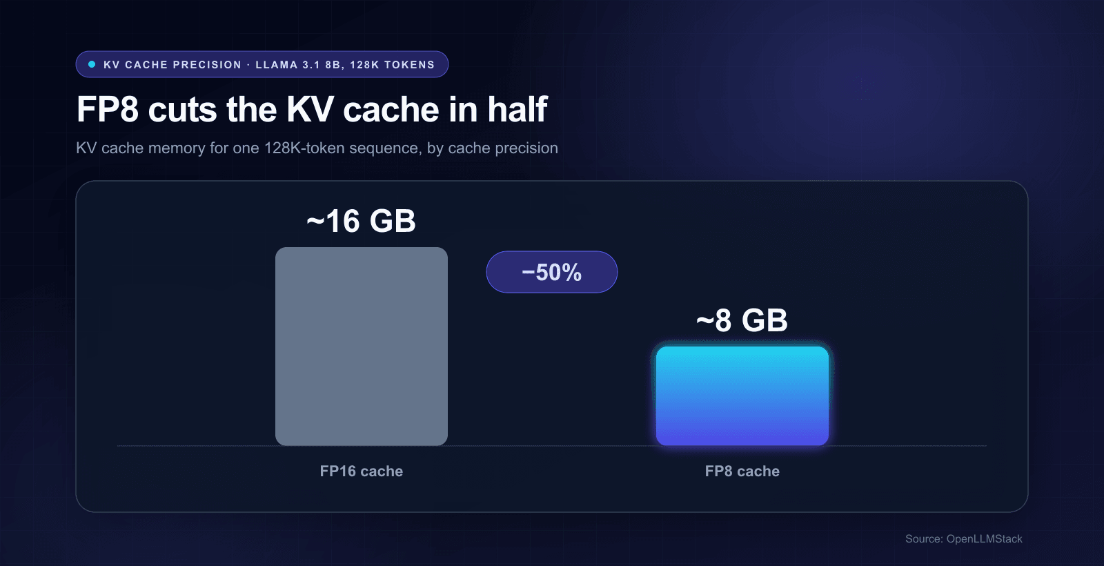
vllm serve meta-llama/Llama-3.1-8B-Instruct --kv-cache-dtype fp8

That single change roughly halves the KV cache footprint, so you can fit a bigger batch or a longer context on the same GPU. SGLang, TensorRT-LLM, and llama.cpp expose similar controls.

The takeaway for anyone self-hosting: you do not have to implement KV caching yourself, but you should tune it. PagedAttention, an FP8 cache, and prefix caching together can multiply the throughput you get from the same hardware.

Frequently asked questions

What is a KV cache in simple terms?

A KV cache is the short-term memory an LLM uses while it writes a response. It saves the key and value vectors for tokens the model has already seen, so the model can reuse them instead of recomputing them for every new token. That reuse is what makes text generation fast.

How does KV caching speed up an LLM?

KV caching lets the model compute keys and values once per token. For each new token, the model appends one new key-value pair per layer and reuses the stored pairs from the existing context. The model still attends over the cached history, so longer contexts continue to increase decode work.

How much memory does a KV cache use?

Enough to rival the model weights. For Llama 3.1 8B at FP16, the KV cache is about 128 KB per token, so one 131,072-token sequence needs roughly 16 GiB. You can calculate it with 2 × layers × kv_heads × head_dim × sequence_length × batch_size × bytes_per_element.

What is KV cache quantization?

KV cache quantization stores attention keys and values at lower precision. Moving from FP16 or BF16 to FP8 roughly halves logical cache memory. Quality and speed effects depend on the numeric format, scaling method, model, hardware, and attention backend.

Does the KV cache change the model output?

No, not by itself. A standard KV cache produces the exact same tokens as recomputing everything from scratch, because the stored keys and values are identical. Output can shift only when you add lossy techniques on top, such as aggressive quantization, eviction, or compression, and even then the effect is usually small.

Final takeaway

KV caching removes one of the largest sources of repeated work in autoregressive LLM inference. The tradeoff is memory. Cache demand rises with layers, active tokens, key-value heads, precision, and concurrency.

If you plan to self-host LLMs, start with the memory formula. Then choose the optimization that matches the bottleneck: PagedAttention for allocation efficiency, FP8 for lower bytes per token, prefix caching for repeated prompts, or offloading for capacity beyond local GPU memory.